Token Supply Modeling: Stress-Test Before You Lock the Contracts

Token supply modeling is the process of projecting how circulating supply, treasury balance, emissions, and buy and sell pressure evolve over time under different scenarios. A Monte Carlo simulation, for example, runs thousands of those scenarios with randomized demand inputs and returns a probability distribution of outcomes at each time horizon, month 6, month 12, month 24, and beyond.

Most founders treat tokenomics design as a one-time document. They negotiate vesting schedules, define emissions, and commit those parameters to smart contracts without ever modeling what happens to supply under adverse conditions. Token supply modeling is the step between "we designed our tokenomics" and "we are confident enough to lock in the contracts."

The revenue-first principle applies here more than anywhere else in the design process. A token supply model is only as credible as the revenue and demand assumptions underneath it. A model with zero revenue inputs is a sophisticated way to confirm that the token has no floor. Model the supply and the business mechanics together, or the output is decoration.

This guide covers the three modeling methods practitioners use, the inputs each method requires, five supply failure patterns modeling catches before launch, and when to commission a specialist engagement rather than run the analysis in-house.

#What Token Supply Modeling Actually Is (And Why It Differs from Tokenomics Design)

Token supply modeling: A simulation methodology that projects the evolution of a protocol's circulating supply, treasury balance, token emissions, and buy/sell pressure under multiple demand scenarios to identify structural failure risks before launch.

Tokenomics design produces the architecture: the allocation table, the vesting schedule, the emissions curve, the burn mechanism if any, the staking yield structure. Token supply modeling simulates whether that architecture survives over time.

The design document states the plan. The model asks what the plan produces under scenarios the design document never tests.

Consider what a standard tokenomics document typically includes. It will show a supply schedule with vesting cliffs by stakeholder class. It will show an emissions curve with month-by-month token release. It might include a simple projection of circulating supply at six months and twelve months. What it rarely includes is a stress test, what happens to treasury balance when demand comes in at the 10th percentile, what happens to token price behavior when investor unlocks at month 12 coincide with a bear market, what happens to staking yield when protocol revenue falls 40% below the base-case assumption.

Token supply modeling fills that gap. The inputs are the design document plus demand assumptions plus scenario variables. The output is a probability distribution, not a single projection line.

Token inflation modeling is one dimension of this work: projecting how emissions relative to demand growth affect purchasing power in the token over time. The others are treasury runway (when does the treasury deplete under the worst-realistic scenario), circulating supply concentration (who holds what share at which unlock events), and sell pressure timing (when do the largest positions become liquid and under what conditions do holders typically sell).

Most tokenomics frameworks treat these as separate analyses. They are one system.

#The Three Methods: Monte Carlo, Agent-Based, and cadCAD

Three methods dominate token supply modeling in practice. They differ in complexity, in what they model well, and in the team resources they require.

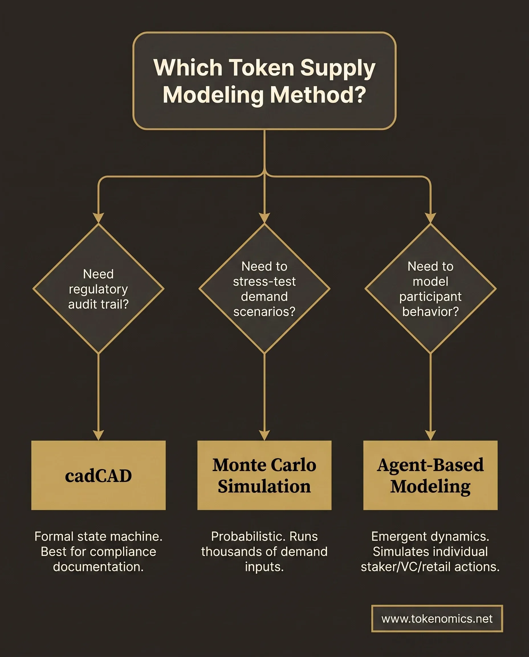
Monte Carlo simulation is the featured method for most founder use cases. A Monte Carlo simulation runs thousands of iterations of your supply model, each time sampling from a distribution of demand inputs rather than using a point estimate. The output is a probability distribution of circulating supply, treasury balance, and key financial ratios at each time horizon. What it models well: probability of treasury depletion, inflation bands under demand uncertainty, sell-pressure concentration at cliff events. What it does not model: strategic behavior by individual participants, emergent dynamics in DeFi liquidity pools, or protocol-revenue feedback loops that change as supply conditions shift.

The appeal of Monte Carlo tokenomics is that it requires only a spreadsheet and basic probability distributions. A founder with a vesting schedule, a revenue-growth assumption, and an estimate of sell pressure per stakeholder class can run a meaningful Monte Carlo in Python or Google Sheets in a day. The questions it answers are the ones that matter most pre-launch: what is the probability our treasury is still solvent at month 24, and what does circulating supply look like in the bottom-decile demand scenario.

Agent-Based Modeling (ABM) simulates individual participants making decisions under defined rules. Holders, stakers, sellers, and arbitrageurs each follow behavioral rules, and the simulation tracks what emerges when those rules interact at scale. ABM is the right method for modeling emergent dynamics: staking and unstaking loops, liquidity pool behavior under stressed conditions, and death-spiral mechanics in yield-farming designs. Chaos Labs uses ABM extensively for DeFi risk analysis. For most pre-launch founder teams without modeling resources, ABM is more complex to build and interpret than the questions justify.

cadCAD (complex adaptive dynamics Computer Aided Design) is a Python-based system-dynamics framework developed by block.science for formal continuous-state-machine modeling. It is the method of choice for regulatory-grade audit trails, for protocols with multi-variable systems, and for complex DeFi mechanism simulation where the math needs to be fully documented and reproducible. The learning curve is steep. Most DeFi protocol teams that use cadCAD have a dedicated token engineering function. For a founder six months from launch trying to stress-test their emissions schedule, cadCAD is likely overkill.

Decision framework by use case:

• Simple supply schedule (up to four stakeholder classes, linear emissions, no DeFi composability): Monte Carlo in a spreadsheet
• DeFi protocol with liquidity pools, staking loops, or yield-farming mechanics: ABM with a specialist team
• Regulatory-grade documentation or a formal mechanism design audit: cadCAD with a token engineering firm

Most founders pre-launch need the first. Most DeFi protocols building ongoing mechanism analysis need the second or third.

#What Your Token Supply Model Actually Needs as Inputs

Token supply modeling is only as useful as its inputs. The demand-side inputs are where most models fail.

Supply-side inputs are typically well-documented in the tokenomics design package:

• Total supply and initial circulating supply at TGE
• Vesting schedule by stakeholder class (team, investors, advisors, treasury, community)
• Cliff dates and unlock schedule for each class
• Emissions schedule for ecosystem rewards, staking, and any protocol incentive programs
• Burn mechanisms and the triggering conditions if any
• Staking lockup ratios and the expected percentage of supply staked at each time horizon

Demand-side inputs are where founders substitute wishful thinking for distributions:

• User growth rate: not a single number but a distribution from pessimistic to base to optimistic
• Revenue per active user or per protocol transaction, grounded in comparable protocol benchmarks
• Sell pressure coefficient per stakeholder class: what percentage of unlocked tokens do investors typically sell in the first 30, 60, and 90 days after a cliff? You can pull the raw post-unlock transfer data from on-chain analytics platforms like Dune Analytics and Nansen. Run the numbers yourself and the picture is rarely flattering. In our experience, investors sell a higher share than founders tend to model for.
• Market condition scenarios: flat, bear, bull, and the tail scenario (severe bear)

Scenario variables complete the model:

• Treasury spending rate (operating costs, grants, ecosystem incentives)
• Protocol revenue versus projections at each time horizon under each demand scenario
• Liquidity depth assumptions if the protocol depends on DEX liquidity for token price stability

The question is never "what is our expected demand." That produces a single projection line that is almost always wrong. The question is "what does our treasury look like in the bottom-10th-percentile demand scenario, and do we still exist at month 24?" That is token economic scenario planning at its most practical.

Review how the allocation table and vesting schedule are structured in the token distribution model before you finalize your supply-side inputs.

#Five Supply Failure Patterns Token Modeling Catches Before Launch

We have seen these patterns repeat across projects. They are not unusual edge cases. They are what happens when the supply architecture is not stress-tested before launch.

1. Treasury runway cliff. The model shows the treasury solvent at month 12. What the model misses until you run the stress test: team and advisor unlocks at month 12 create a concentrated sell window the treasury cannot absorb through buybacks at any price above the 10th-percentile scenario. By month 18, the treasury is near zero. This is not theoretical risk. Most projects where this occurs do not get a second chance to fix it post-launch.

2. Circular staking death spiral. Staking yield is funded by emissions rather than protocol revenue. The model shows attractive APY through month 18. The stress test reveals the mechanism's fragility: as token price falls, APY in dollar terms collapses; stakers unstake; sell pressure accelerates; price falls further. The loop has no revenue floor to interrupt it. We've seen this pattern in projects where staking was designed to reduce sell pressure without asking whether the protocol had the revenue to sustain the yield.

3. Unlock concentration front-run. Investors hold 30 to 40% of supply in a single stakeholder class. The cliff is at month 12. In the model with optimistic demand inputs, this looks manageable. When you run the scenario with realistic sell pressure coefficients, informed market participants begin accumulating short positions 60 to 90 days before the cliff. The unlock window becomes the price event the founder did not model. Modeling this window 18 months before launch is actionable; modeling it after launch is just analysis.

4. Token inflation modeling reveals emissions outpacing demand. The emissions schedule requires 8 to 12% year-over-year demand growth to maintain price equilibrium. The Monte Carlo simulation at 2 to 4% demand growth (which matches the baseline for most new protocols in their first two years) shows a supply overhang that compresses token price by month 18. The design assumed demand would grow into emissions. The model shows the timing doesn't work.

5. Community pool depletion ahead of schedule. Community allocations are modeled to last 36 months, funding grants, ecosystem incentives, and growth programs. When you benchmark the actual spend rate against comparable protocols, using treasury and revenue figures you can pull from Token Terminal and public protocol disclosures, the community pool often depletes in 18 to 24 months. That eliminates the growth flywheel at the moment it should be paying off.

Every failure pattern above is a mismatch between supply growth and the underlying business's ability to create revenue-backed demand. The model quantifies when the mismatch becomes fatal. Stress testing before launch is what converts a design document into a plan that can hold up under scrutiny.

#Running Your First Monte Carlo Token Supply Simulation

The mechanics of token supply modeling are less daunting than they sound. You need three things: your supply schedule in a spreadsheet, probability distributions for your key demand inputs, and a basic Monte Carlo framework.

Tooling options by complexity:

• Google Sheets or Excel with Monte Carlo add-ins (Crystal Ball, @RISK): appropriate for supply models with up to four stakeholder classes and linear emissions
• Python with NumPy and pandas: appropriate for more complex models or when you want full auditability and reproducibility; basic Monte Carlo in Python is 50 to 100 lines of code
• Specialist platforms (Gauntlet for DeFi risk, Chaos Labs for agent-based, Tokenomics.net for pre-launch founder engagements): appropriate when model complexity exceeds what a general engineering team can manage or when the output needs to hold up under investor or regulatory scrutiny

How to read the output:

Instead of a single projection line, a Monte Carlo produces a cone of outcomes at each time horizon. The 10th percentile is the stress test. The 50th percentile is the base case. The 90th percentile is the optimistic scenario. The width of the cone tells you how sensitive your model is to demand assumptions.

Each scenario is defined by a coherent set of supply parameters, not a single tweaked number. Move them together. Here is what a representative three-scenario setup looks like across the five parameters that drive most supply outcomes. The values below are illustrative, not benchmarks; your own design and comparable-protocol data set the real numbers.

Supply parameter	Bull (90th pct)	Base (50th pct)	Stress (10th pct)
Emission rate (annual, % of supply)	4%	7%	11%
Vesting cliff sell-through (first 90 days)	20% sold	45% sold	75% sold
Treasury burn rate (monthly operating draw)	1.5%	2.5%	4%
Staking lock ratio (supply staked at 12mo)	55%	35%	15%
Circulating supply at 12 months (% of total)	28%	41%	58%

Read the table as three internally consistent worlds. In the stress column, emissions run hot, investors dump most of their unlock, the treasury bleeds faster, almost nothing stays staked, and circulating supply balloons past the halfway mark inside a year. That is the combination token supply modeling exists to surface before you commit the parameters to a contract.

Red flags in the output that require design revision before launch:

• 10th percentile scenario shows treasury depletion before month 18
• Circulating supply at month 12 exceeds 50% of FDV in the base case (50th percentile), which signals concentrated unlock risk in the near term
• Staking yield in dollar terms falls below protocol's own competing yields in any bear scenario, signaling the mechanism depends on price not revenue
• Community pool depletion occurs before month 24 at base-case spending rates

If any of these appear in your token supply modeling run, the design needs revision. That revision is far less expensive before launch than after. The tokenomics audit checklist covers the seven dimensions you should validate before concluding the supply model is sound.

#When to Commission a Token Supply Modeling Engagement

There is a line between what a founder can run in-house and what requires a specialist engagement. It runs at model complexity.

Token supply modeling you can run in-house: up to four stakeholder classes, linear vesting with standard cliffs, simple emissions curve, no DeFi composability, no protocol-revenue feedback loops. Monte Carlo in a spreadsheet or in basic Python is sufficient.

A supply model that benefits from a specialist engagement: more than four stakeholder classes, non-linear emissions that respond to protocol revenue or staking ratios, DeFi composability (liquidity pools, yield farming, staking and unstaking loops), or a design that needs to hold up under investor due diligence or regulatory review.

What a specialist modeling engagement produces is different from an internal analysis. The outputs include scenario analysis with 1,000 to 10,000 Monte Carlo iterations across your full demand distribution, a failure-pattern report identifying specific design vulnerabilities with revision recommendations, and documentation formatted to answer the questions institutional investors ask (the treasury runway question, the circulating supply concentration question, the sell pressure question).

The timing matters too. Token supply modeling should happen before vesting schedule negotiations with investors are complete. Modeling done after investor terms are locked has limited room to revise the largest supply-side risk in the design. Get the model right while you still have negotiating room.

Your house needs to be in order before you go to market. That means knowing what your supply looks like in the bottom-decile scenario before you pitch, not after you've committed.

#Frequently Asked Questions

What is the difference between token supply modeling and tokenomics design?

Tokenomics design is the process of specifying a token's supply architecture: the allocation table, vesting schedule, emissions curve, utility sinks, and burn mechanics. Token supply modeling is a simulation step that takes those specifications as inputs and projects how circulating supply, treasury balance, and sell pressure evolve over multiple time horizons under different demand scenarios. Design produces the plan. Modeling stress-tests the plan before any parameters are locked into smart contracts.

When should founders run a Monte Carlo simulation for tokenomics?

Founders should run a Monte Carlo token supply simulation before investor vesting negotiations are complete and before supply parameters are committed to smart contracts. The optimal window is three to six months before TGE: early enough that the design is defined enough to model, late enough that the parameters reflect realistic investor and community allocations. Re-run whenever the supply schedule changes materially.

What inputs does a token supply model require to be useful?

A token supply model requires three categories of inputs: (1) supply-side inputs from the tokenomics design document, including total supply, vesting schedule by stakeholder class, emissions curve, and burn conditions; (2) demand-side inputs as probability distributions rather than single point estimates, including user growth rate range, revenue per active user, and sell pressure coefficient per stakeholder class based on on-chain comparables; and (3) scenario variables, including market condition assumptions (bull/flat/bear/tail), treasury spending rate, and liquidity depth assumptions for DEX-dependent models.

What is treasury runway in tokenomics?

Treasury runway is the number of months a protocol's treasury can fund operations, grants, and ecosystem incentives before it depletes, measured under a specific demand and spending scenario rather than as a single headline figure. The number that matters is not runway in the base case. It is runway in the bottom-decile scenario, when revenue underperforms and a token-denominated treasury loses value at the same time. Token supply modeling computes runway across the full distribution so you see when the treasury hits zero in the worst realistic conditions, not just the comfortable ones.

How do vesting cliffs affect token price?

A vesting cliff releases a concentrated block of previously locked tokens to a stakeholder class on a single date, which creates a predictable sell window the market can see coming. When investor and team cliffs land together, the supply that becomes liquid in one window can swamp available demand, and informed participants often position ahead of the unlock. This is one of the clearest things token supply modeling catches: it overlays cliff dates against projected demand and treasury buyback capacity, so you know whether a given cliff is a non-event or a price cliff before the contract locks the schedule.

What tools do tokenomics consultants use for supply modeling?

Most pre-launch token supply modeling runs on three methods. Monte Carlo simulation in Python or a spreadsheet handles probabilistic scenario analysis and covers the majority of founder use cases. Agent-based modeling simulates individual participant behavior for emergent dynamics like staking loops and DeFi liquidity effects. cadCAD provides formal, reproducible system-dynamics modeling for regulatory-grade audit trails. Raw on-chain inputs (unlock transfers, treasury balances, staking ratios) are pulled from analytics platforms like Dune Analytics, Nansen, and Token Terminal, then fed into whichever modeling method fits the protocol's complexity.

---

The projects that survive a bear market, an investor cliff, or a community frustration cycle are the ones that stress-tested these scenarios before launch. A token supply model is not a prediction. It is a due diligence step that converts "we hope this works" into "we know what it looks like if it doesn't, and we've designed for that."

If you are building onchain and need your token supply model to hold up under investor scrutiny, book a discovery call. We will assess your supply architecture and tell you whether we are the right fit. Sometimes we're not. We'll tell you that too.

If you need the full documentation package alongside the model, our data room service covers the complete supply model, distribution plan, and investor-grade documentation in one engagement.